A Story of Basis and Kernel - Part II: Reproducing Kernel Hilbert Space

1. Opening Words

In the previous blog, the function basis was briefly discussed. We began with viewing a function as an infinite vector, and then defined the inner product of functions. Similar to $\mathcal{R}^n$ space, we can also find orthogonal function basis for a function space.

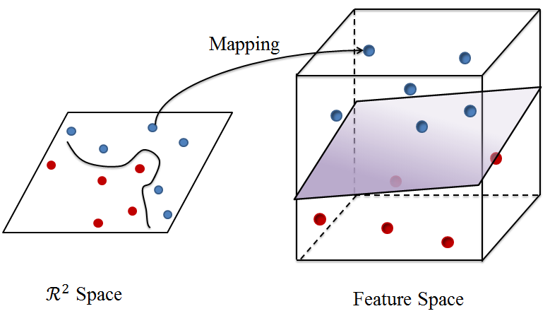
This blog will move a step further discussing about kernel functions and reproducing kernel Hilbert space (RKHS). Kernel methods have been widely used in a variety of data analysis techniques. The motivation of kernel method arises in mapping a vector in $\mathcal{R}^n$ space as another vector in a feature space. For example, imagine there are some red points and some blue points as the next figure shows, which are not easily separable in $\mathcal{R}^n$ space. However, if we map them into a high-dimension feature space, we may be able to seperate them easily. This article will not provide strict theoretical definition, but rather intuitive description on the basic ideas.

2. Eigen Decomposition

For a real symmetric matrix $\mathbf{A}$ , there exists real number $\lambda$ and vector $\mathbf{x}$ so that

$\mathbf{A} \mathbf{x} = \lambda \mathbf{x}$

Then $\lambda$ is an eigenvalue of $\mathbf{A}$ and $\mathbf{x}$ is the corresponding eigenvector. If $\mathbf{A}$ has two different eigenvalues $\lambda_1$ and $\lambda_2$ , $\lambda_1 \neq \lambda_2$ , with corresponding eigenvectors $\mathbf{x}_1$ and $\mathbf{x}_2$ respectively,

$\lambda_1 \mathbf{x}_1^T \mathbf{x}_2 = \mathbf{x}_1^T \mathbf{A}^T \mathbf{x}_2 = \mathbf{x}_1^T \mathbf{A} \mathbf{x}_2 = \lambda_2 \mathbf{x}_1^T \mathbf{x}_2$

Since $\lambda_1 \neq \lambda_2$ , we have $\mathbf{x}_1^T \mathbf{x}_2 = 0$ , i.e., $\mathbf{x}_1$ and $\mathbf{x}_2$ are orthogonal.

For $\mathbf{A} \in \mathcal{R}^{n \times n}$ , we can find $n$ eigenvalues a long with $n$ orthogonal eigenvectors. As a result, $\mathbf{A}$ can be decomposited as

$\mathbf{A} = \mathbf{Q} \mathbf{D} \mathbf{Q}^T$

where $\mathbf{Q}$ is an orthogonal matrix (i.e., $\mathbf{Q} \mathbf{Q}^T = \mathbf{I}$ ) and $\mathbf{D} = \text{diag} (\lambda_1, \lambda_2, \cdots, \lambda_n)$ . If we write $\mathbf{Q}$ column by column

$\mathbf{Q}=\left( \mathbf{q}_1, \mathbf{q}_2, \cdots, \mathbf{q}_n \right)$

then

$\begin{array}{rl} \mathbf{A}=\mathbf{Q} \mathbf{D} \mathbf{Q}^T &= \left( \mathbf{q}_1, \mathbf{q}_2, \cdots, \mathbf{q}_n \right) \begin{pmatrix} \lambda_1\ &&& \\ & \lambda_2\ && \\ && \ddots\ & \\ &&&\lambda_n \end{pmatrix} \begin{pmatrix} \mathbf{q}_1^T \\ \mathbf{q}_2^T \\ \vdots \\ \mathbf{q}_n^T \end{pmatrix} \\ &= \left( \lambda_1 \mathbf{q}_1, \lambda_2 \mathbf{q}_2, \cdots, \lambda_n \mathbf{q}_n \right) \begin{pmatrix} \mathbf{q}_1^T \\ \mathbf{q}_2^T \\ \vdots \\ \mathbf{q}_n^T \end{pmatrix} \\ &=\sum_{i=1}^n \lambda_i \mathbf{q}_i \mathbf{q}_i^T \end{array}$

Here ${ \{\mathbf{q}_i \} }_{i=1}^n$ is a set of orthogonal basis of $\mathcal{R}^n$ .

3. Kernel Function

A function $f(\mathbf{x})$ can be viewed as an infinite vector, then for a function with two independent variables $K(\mathbf{x},\mathbf{y})$ , we can view it as an infinite matrix. Among them, if $K(\mathbf{x},\mathbf{y}) = K(\mathbf{y},\mathbf{x})$ and

$\int \int f(\mathbf{x}) K(\mathbf{x},\mathbf{y}) f(\mathbf{y}) d\mathbf{x} d\mathbf{y} \geq 0$

for any function $f$ , then $K(\mathbf{x},\mathbf{y})$ is symmetric and positive definite, in which case $K(\mathbf{x},\mathbf{y})$ is a kernel function.

Similar to matrix eigenvalue and eigenvector, there exists eigenvalue $\lambda$ and eigenfunction $\psi(\mathbf{x})$ so that

$\int K(\mathbf{x},\mathbf{y}) \psi(\mathbf{x}) d\mathbf{x} = \lambda \psi(\mathbf{y})$

For different eigenvalues $\lambda_1$ and $\lambda_2$ with corresponding eigenfunctions $\psi_1(\mathbf{x})$ and $\psi_2(\mathbf{x})$ , it is easy to show that

$\begin{array}{rl} \int \lambda_1 \psi_1(\mathbf{x}) \psi_2(\mathbf{x}) d\mathbf{x} & = \int \int K(\mathbf{y},\mathbf{x}) \psi_1(\mathbf{y}) d\mathbf{y} \psi_2(\mathbf{x}) d\mathbf{x} \\ & = \int \int K(\mathbf{x},\mathbf{y}) \psi_2(\mathbf{x}) d\mathbf{x} \psi_1(\mathbf{y}) d\mathbf{y} \\ & = \int \lambda_2 \psi_2(\mathbf{y}) \psi_1(\mathbf{y}) d\mathbf{y} \\ & = \int \lambda_2 \psi_2(\mathbf{x}) \psi_1(\mathbf{x}) d\mathbf{x} \end{array}$

Therefore,

$< \psi_1, \psi_2 > = \int \psi_1(\mathbf{x}) \psi_2(\mathbf{x}) d\mathbf{x} = 0$

Again, the eigenfunctions are orthogonal. Here $\psi$ denotes the function (the infinite vector) itself.

For a kernel function, infinite eigenvalues ${ \{\lambda_i\} }_{i=1}^{\infty}$ along with infinite eigenfunctions ${ \{\psi_i\} }_{i=1}^{\infty}$ may be found. Similar to matrix case,

$K(\mathbf{x},\mathbf{y}) = \sum_{i=0}^{\infty} \lambda_i \psi_i (\mathbf{x}) \psi_i (\mathbf{y})$

which is the Mercer's theorem. Here $< \psi_i, \psi_j > = 0$ for $i \neq j$ . Therefore, ${ \{\psi_i\} }_{i=1}^{\infty}$ construct a set of orthogonal basis for a function space.

Here are some commonly used kernels:

• Polynomial kernel $K(\mathbf{x},\mathbf{y}) = ( \gamma \mathbf{x}^T \mathbf{y} + C)^d$
• Gaussian radial basis kernel $K(\mathbf{x},\mathbf{y}) = \exp (-\gamma \Vert \mathbf{x} - \mathbf{y} \Vert^2 )$
• Sigmoid kernel $K(\mathbf{x},\mathbf{y}) = \tanh (\gamma \mathbf{x}^T \mathbf{y} + C )$

4. Reproducing Kernel Hilbert Space

Treat ${ \{\sqrt{\lambda_i} \psi_i\} }_{i=1}^{\infty}$ as a set of orthogonal basis and construct a Hilbert space $\mathcal{H}$ . Any function or vector in the space can be represented as the linear combination of the basis. Suppose

$f = \sum_{i=1}^{\infty} f_i \sqrt{\lambda_i} \psi_i$

we can denote $f$ as an infinite vector in $\mathcal{H}$ :

$f = (f_1, f_2, ...)_\mathcal{H}^T$

For another function $g = (g_1, g_2, ...)_\mathcal{H}^T$ , we have

$< f,g >_\mathcal{H} = \sum_{i=1}^{\infty} f_i g_i$

For the kernel function $K$, here I use $K(\mathbf{x},\mathbf{y})$ to denote the evaluation of $K$ at point $\mathbf{x},\mathbf{y}$ which is a scalar, use $K(\cdot,\cdot)$ to denote the function (the infinite matrix) itself, and use $K(\mathbf{x},\cdot)$ to denote the $\mathbf{x}$th "row" of the matrix, i.e., we fix one parameter of the kernel function to be $\mathbf{x}$ then we can regard it as a function with one parameter or as an infinite vector. Then

$K(\mathbf{x},\cdot) = \sum_{i=0}^{\infty} \lambda_i \psi_i (\mathbf{x}) \psi_i$

In space $\mathcal{H}$ , we can denote

$K(\mathbf{x},\cdot) = (\sqrt{\lambda_1} \psi_1 (\mathbf{x}), \sqrt{\lambda_2} \psi_2 (\mathbf{x}), \cdots )_\mathcal{H}^T$

Therefore

$< K(\mathbf{x},\cdot), K(\mathbf{y},\cdot) >_\mathcal{H} = \sum_{i=0}^{\infty} \lambda_i \psi_i (\mathbf{x}) \psi_i(\mathbf{y}) = K(\mathbf{x},\mathbf{y})$

This is the reproducing property, thus $\mathcal{H}$ is called reproducing kernel Hilbert space (RKHS).

Now it is time to return to the problem from the beginning of this article: how to map a point into a feature space? If we define a mapping

$\bold{\Phi} (\mathbf{x}) = K(\mathbf{x},\cdot) = (\sqrt{\lambda_1} \psi_1 (\mathbf{x}), \sqrt{\lambda_2} \psi_2 (\mathbf{x}), \cdots )^T$

then we can map the point $\mathbf{x}$ to $\mathcal{H}$ . Here $\bold{\Phi}$ is not a function, since it points to a vector or a funtion in the feature space $\mathcal{H}$ . Then

$< \bold{\Phi} (\mathbf{x}), \bold{\Phi} (\mathbf{y}) >_\mathcal{H} = < K(\mathbf{x},\cdot), K(\mathbf{y},\cdot) >_\mathcal{H} = K(\mathbf{x},\mathbf{y})$

As a result, we do not need to actually know what is the mapping, where is the feature space, or what is the basis of the feature space. For a symmetric positive-definite function $K$ , there must exist at least one mapping $\bold{\Phi}$ and one feature space $\mathcal{H}$ so that

$< \bold{\Phi} (\mathbf{x}), \bold{\Phi} (\mathbf{y}) > = K(\mathbf{x},\mathbf{y})$

which is the so-called kernel trick.

5. A Simple Example

Consider kernel function

$K(\mathbf{x},\mathbf{y}) = \left( x_1, x_2, x_1 x_2 \right) \begin{pmatrix} y_1 \\ y_2 \\ y_1 y_2 \end{pmatrix} = x_1 y_1 + x_2 y_2 + x_1 x_2 y_1 y_2$

where $\mathbf{x}=(x_1,x_2)^T, \mathbf{y}=(y_1,y_2)^T$ . Let $\lambda_1=\lambda_2=\lambda_3=1$ , $\psi_1(\mathbf{x})=x_1$ , $\psi_2(\mathbf{x})=x_2$ , $\psi_3(\mathbf{x})=x_1 x_2$ . We can define the mapping as

$\begin{pmatrix} x_1 \\ x_2 \end{pmatrix} \overset{\bold{\Phi}}{\longrightarrow} \begin{pmatrix} x_1 \\ x_2 \\ x_1 x_2 \end{pmatrix}$

Then

$< \bold{\Phi} (\mathbf{x}), \bold{\Phi}(\mathbf{y}) > = \left( x_1, x_2, x_1 x_2 \right) \begin{pmatrix} y_1 \\ y_2 \\ y_1 y_2 \end{pmatrix} = K(\mathbf{x},\mathbf{y})$

6. Support Vector Machine

Support vector machine (SVM) is one of the most widely known application of RKHS. Suppose we have data pairs ${ (\mathbf{x}_i, y_i) }_{i=1}^n$ where $y_i$ is either 1 or -1 denoting the class of the point $\mathbf{x}_i$. SVM assumes a hyperplane to best seperate the two classes.

$\min_{\boldsymbol{\beta}, \beta_0} \frac{1}{2} \Vert \boldsymbol{\beta} \Vert^2 + C \sum_{i=1}^n \xi_i$

$\text{subject to } \xi_i \geq 0, y_i (\mathbf{x}_i^T \boldsymbol{\beta} + \beta_0 ) \geq 1 - \xi_i, \forall i$

Sometimes the two classes cannot be easily seperated in $\mathcal{R}^n$ space, thus we can map $\mathbf{x}_i$ into a high-dimension feature space where the two classes may be easily seperated. The original problem can be reformulated as

$\min_{\boldsymbol{\beta}, \beta_0} \frac{1}{2} \Vert \boldsymbol{\beta} \Vert^2 + C \sum_{i=1}^n \xi_i$

$\text{subject to } \xi_i \geq 0, y_i (\bold{\Phi}(\mathbf{x}_i)^T \boldsymbol{\beta} + \beta_0 ) \geq 1 - \xi_i, \forall i$

The Lagrange function is

$L_p = \frac{1}{2} \Vert \boldsymbol{\beta} \Vert^2 + C \sum_{i=1}^n \xi_i - \sum_{i=1}^n \alpha_i [y_i (\bold{\Phi}(\mathbf{x}_i)^T \boldsymbol{\beta} + \beta_0) - (1-\xi_i)] -\sum_{i=1}^n \mu_i \xi_i$

Since

$\frac{\partial L_p}{\partial \boldsymbol{\beta}} = \mathbf{0}$

we get

$\boldsymbol{\beta} = \sum_{i=1}^n \alpha_i y_i \bold{\Phi}(\mathbf{x}_i)$

That is, $\boldsymbol{\beta}$ can be writen as the linear combination of $\mathbf{x}_i$s! We can substitute $\boldsymbol{\beta}$ and get the new optimization problem. The objective function changes to:

$\begin{array}{rl} &\frac{1}{2} \Vert \sum_{i=1}^n \alpha_i y_i \bold{\Phi} (\mathbf{x}_i) \Vert^2 + C \sum_{i=1}^n \xi_i \\ =& \frac{1}{2} < \sum_{i=1}^n \alpha_i y_i \bold{\Phi} (\mathbf{x}_i), \sum_{j=1}^n \alpha_j y_j \bold{\Phi} (\mathbf{x}_j) > + C \sum_{i=1}^n \xi_i \\ =& \frac{1}{2} \sum_{i=1}^n \sum_{j=1}^n \alpha_i \alpha_j y_i y_j < \bold{\Phi} (\mathbf{x}_i), \bold{\Phi} (\mathbf{x}_j) > + C \sum_{i=1}^n \xi_i \\ = & \frac{1}{2} \sum_{i=1}^n \sum_{j=1}^n \alpha_i \alpha_j y_i y_j K(\mathbf{x}_i, \mathbf{x}_j) + C \sum_{i=1}^n \xi_i \end{array}$

The constraints changes to:

$\begin{array}{rl} & y_i \left[\bold{\Phi}(\mathbf{x}_i)^T \left( \sum_{j=1}^n \alpha_j y_j \bold{\Phi}(\mathbf{x}_j) \right) + \beta_0 \right] \\ =& y_i \left[ \left( \sum_{j=1}^n \alpha_j y_j < \bold{\Phi}(\mathbf{x}_i), \bold{\Phi}(\mathbf{x}_j) > \right) + \beta_0 \right] \\ =& y_i \left[ \left( \sum_{j=1}^n \alpha_j y_j K(\mathbf{x}_i, \mathbf{x}_j) \right) + \beta_0 \right] \geq 1 - \xi_i, \forall i \end{array}$

What we need to do is determining a kernel function and solve for $\boldsymbol{\alpha}, \beta_0, \xi_i$ . We do not need to actually construct the feature space. For a new data $\mathbf{x}$ with unknown class, we can predict its class by

$\begin{array}{ccl} \hat{y} &=& \text{sign} \left[ \bold{\Phi} (\mathbf{x})^T \boldsymbol{\beta} + \beta_0 \right] \\ &=& \text{sign} \left[ \bold{\Phi} (\mathbf{x})^T \left( \sum_{i=1}^n \alpha_i y_i \bold{\Phi}(\mathbf{x}_i) \right) + \beta_0 \right] \\ &=& \text{sign} \left( \sum_{i=1}^n \alpha_i y_i < \bold{\Phi} (\mathbf{x}), \bold{\Phi}(\mathbf{x}_i) > + \beta_0 \right) \\ &=& \text{sign} \left( \sum_{i=1}^n \alpha_i y_i K(\mathbf{x},\mathbf{x}_i) + \beta_0 \right) \end{array}$

Kernel methods greatly strengthen the discriminative power of SVM.

7. Summary and Reference

Kernel method has been widely utilized in data analytics. Here, the fundamental property of RKHS is introduced. With kernel trick, we can easily map the data to a feature space and do analysis. Here is a video with nice demonstration on why we can easily do classification with kernel SVM in a high-dimension feature space.

The example in Section 5 is from

• Gretton A. (2015): Introduction to RKHS, and some simple kernel algorithms, Advanced Topics in Machine Learning, Lecture conducted from University College London.

Other reference includes

• Paulsen, V. I. (2009). An introduction to the theory of reproducing kernel Hilbert spaces. Lecture Notes.
• Daumé III, H. (2004). From zero to reproducing kernel hilbert spaces in twelve pages or less.
• Friedman, J., Hastie, T., and Tibshirani, R. (2001). The elements of statistical learning. Springer, Berlin: Springer series in statistics.)